Matlab Level 12 For Engineers in Planes automobile trrains applications by Mr.MA 2018

Matlab-Simulink

----------------------------

Introduction :

Matlab Simulink use in many fields in signals analysis,

Systems, transfere functions, Digital systems, Planes,

Digital cameras and sensors and soon….

Firstly : I show you some Matlab Simulink Boxes :

1-A

++++++++++++++++++++++++++++++++++++++++++++++++++
+++++++++++++++++++++++++++++++++++++++++++++++++
+++++++++++++++++++++++++++++++++++++++++++++++

Matlab Simulink

----------------------------

Εισαγωγή:

Το Matlab Simulink χρησιμοποιεί πολλά πεδία στην ανάλυση σήματος,
Συστήματα, λειτουργίες μεταβίβασης, ψηφιακά συστήματα, σχέδια,
Ψηφιακές κάμερες και αισθητήρες και σύντομα ....

Πρώτον: Σας παρουσιάζω κάποια κουτιά

Matlab Simulink:

1-Α

                                                                   Fig-1

Here there are many libraries consist each of them of many boxes 

and electrical electronics components and devices.

Example : HDL Coder ;

Can transfer all the components and the system architecture with 

it’s simulations in HDL Files, …

Another example continous libraries you will find DC Sources, AC 

sources, continous source signals and so on.

So  finally each library consists of electrical-electronic components 

and devices for electrical treatements and architecturesin all 

engineering fields as trains control circuits, cars signal analysis, 

planes and calculators architectures and so on……

****************************************************************
Ακολουθούν πολλές βιβλιοθήκες και ηλεκτρικών ηλεκτρονικών εξαρτημάτων και συσκευών.

Παράδειγμα: κωδικοποιητής HDL.

Μπορεί να μεταφέρει όλα τα στοιχεία και την αρχιτεκτονική του συστήματος με
είναι προσομοιώσεις σε αρχεία HDL, ...

Ένα άλλο παράδειγμα συνεχών βιβλιοθηκών που θα βρείτε είναι οι πηγές DC AC
πηγές, συνεχή σήματα πηγής και ούτω καθεξής.


Έτσι κάθε βιβλιοθήκη αποτελείται από ηλεκτρο-ηλεκτρονικά εξαρτήματα
και συσκευές για ηλεκτρικές επεξεργασίες και αρχιτεκτονικέ

πεδία τεχνικών όπως κυκλώματα ελέγχου αμαξοστοιχιών, ανάλυση σήματος αυτοκινήτων,

αρχιτεκτονικές σχεδίου και αριθμομηχανών και ούτω καθεξής ......

****************************************************************

  

Fig-2

                                                 This second  Example show us

Another libraries and another boxes findinside Matlab Simulink.

Αυτό το δεύτερο παράδειγμα μας δείχνει

Άλλες βιβλιοθήκες και άλλα κουτιά βρίσκουν το Matlab Simulink.

1-C 

Fig-3

1-4

Fig-4

++++++++++++++++++++++++++++++++++++++++++++++++++++++++++++++++++++++++++++++++++++++++++++++++++++++++++++++++++++++++++++++++++++++++++++++++++++++++++++++++++++++++++++++++++++++++++

 

 2- Applications in Matlab :

Applications For image processing in the fields of medicine or research or spatial or electronics architectures and sensors developpements……. specailly in image processing.

Εφαρμογές Για την επεξεργασία εικόνων στον τομέα της ιατρικής ή της έρευνας ή της χωρικής αρχιτεκτονικής και των αισθητήρων ....... specailly στην επεξεργασία εικόνας.

Registering an Image Using Normalized Cross-Correlation

This example shows how to find a template image within a larger image.

Sometimes one image is a subset of another. Normalized cross-correlation can be used to determine how to register or align, or modifing the images by translating, translation methods one of them.

We here show how to read an image file , file name type png,….

Αυτό το παράδειγμα δείχνει πώς μπορείτε να βρείτε μια εικόνα προτύπου σε μια μεγαλύτερη εικόνα.

Μερικές φορές μια εικόνα είναι ένα υποσύνολο άλλου. Η κανονικοποιημένη συσχέτιση μπορεί να χρησιμοποιηθεί για τον προσδιορισμό του τρόπου εγγραφής ή ευθυγράμμισης ή τροποποίησης των εικόνων μεταφράζοντας τις μεθόδους μετάφρασης σε μία από αυτές.

Δείχνουμε πώς να διαβάζουμε ένα αρχείο εικόνας, όνομα αρχείου png,

Step 1: Read Image

onion = imread('onion.png');

peppers = imread('peppers.png');

imshow(onion)

figure, imshow(peppers)

                                                                     Fig-5

Fig-6

Step 2: Choose Subregions of Each Image

It is important to choose regions that are similar.

The image sub_onion will be the template, and must be smaller than the image sub_peppers. You can get these sub regions using either the non-interactive script below or the interactive script.

You can use here the methods non-interactive or the other method interactive.

Firstly

% non-interactively

rect_onion = [111 33 65 58];

rect_peppers = [163 47 143 151];

sub_onion = imcrop(onion,rect_onion);

sub_peppers = imcrop(peppers,rect_peppers);

% OR

%Secondly             

% interactively

%[sub_onion,rect_onion] = imcrop(onion); % choose the pepper below the onion

%[sub_peppers,rect_peppers] = imcrop(peppers); % choose the whole onion

% display sub images

figure, imshow(sub_onion)

                          

Fig-7

figure, imshow(sub_peppers)

                            

                             

fig-8

Step 3: Do Normalized Cross-Correlation and Find Coordinates of Peak

Calculate the normalized cross-correlation (Correlations methods in imaging processing and treatements) and display it as a surface plot.

 The peak of the cross-correlation matrix occurs where the sub_images are best correlated. normxcorr2 only works on grayscale images, so we pass it the red plane of each sub image.

c = normxcorr2(sub_onion(:,:,1),sub_peppers(:,:,1));

figure, surf(c), shading flat

Fig-9

Step 4: Find the Total Offset Between the Images

The total offset or translation between images depends on the location of the peak in the cross-correlation matrix, and on the size and position of the sub images.

% offset found by correlation

[max_c, imax] = max(abs(c(:)));

[ypeak, xpeak] = ind2sub(size(c),imax(1));

corr_offset = [(xpeak-size(sub_onion,2))

               (ypeak-size(sub_onion,1))];

% relative offset of position of subimages

rect_offset = [(rect_peppers(1)-rect_onion(1))

               (rect_peppers(2)-rect_onion(2))];

% total offset

offset = corr_offset + rect_offset;

xoffset = offset(1);

yoffset = offset(2);

Step 5: See if the Onion Image was Extracted from the Peppers Image

Figure out where onion falls inside of peppers.

xbegin = round(xoffset+1);

xend   = round(xoffset+ size(onion,2));

ybegin = round(yoffset+1);

yend   = round(yoffset+size(onion,1));

% extract region from peppers and compare to onion

extracted_onion = peppers(ybegin:yend,xbegin:xend,:);

if isequal(onion,extracted_onion)

   disp('onion.png was extracted from peppers.png')

end

onion.png was extracted from peppers.png

Step 6: Pad the Onion Image to the Size of the Peppers Image

Pad the onion image to overlay on peppers, using the offset determined above.

recovered_onion = uint8(zeros(size(peppers)));

recovered_onion(ybegin:yend,xbegin:xend,:) = onion;

figure, imshow(recovered_onion)

Fig-10

Step 7: Use Alpha Blending To Show Images Together

Display one plane of the peppers image with the recovered_onion image using alpha blending.

figure, imshowpair(peppers(:,:,1),recovered_onion,'blend')

Fig-11

Fig-12

+++++++++++++++++++++++++++++++++++++++++++++++++++++++++++++++++++++++++++++++++++++++++++++++++++++++++++++++++++++++++++++++++++++++++++++++++++++++++++++++++++++++++++

3- Applications in Matlab :

Applications For image processing in the fields of medicine or research or spatial or electronics architectures and sensors developpements……. specailly in image processing.

Deblurring Images Using a Regularized Filter

This example shows how to use regularized deconvolution to deblur images.

Regularized deconvolution can be used effectively when constraints are applied on the recovered image (e.g., smoothness, Brightness, …) and limited information is known about the additive noise.

The blurred and noisy image is restored by a constrained least square restoration algorithm that uses a regularized filter (type of regulated digitized filters).

Step 1: Read Image

The example reads in an RGB image and crops it to be 256-by-256-by-3. The deconvregence function can handle arrays of any dimension (10*10,100*100,….1000*1000*1000…..).

I = imread('tissue.png');

I = I(125+(1:256),1:256,:);

f1 = figure;

imshow(I);

figure(f1);

title('Original Image');

text(size(I,2),size(I,1)+15, ...

'Image courtesy of Alan Partin, Johns Hopkins University', ...

'FontSize',7,'HorizontalAlignment','right');

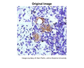
Fig-13

Step 2: Simulate a Blur and Noise

Simulate a real-life image that could be blurred (e.g., due to camera motion or lack of focus) and noisy (e.g., due to random disturbances).

The example simulates the blur by convolving a Gaussian filter with the true image (using imfilter).

The Gaussian filter represents a point-spread function, PSF.

PSF = fspecial('gaussian',11,5);

Blurred = imfilter(I,PSF,'conv');

f2 = figure;

imshow(Blurred);

figure(f2);

title('Blurred');

Fig-14

We simulate the noise by adding a Gaussian noise of variance V to the blurred image (using imnoise).

V = .02;

BlurredNoisy = imnoise(Blurred,'gaussian',0,V);

f3 = figure;

imshow(BlurredNoisy);

figure(f3);

title('Blurred & Noisy');

                                       FIG-15

Step 3: Restore the Blurred and Noisy Image

Restore the blurred and noisy image supplying noise power, NP, as the third input parameter.

 To illustrate how sensitive the algorithm and algortithmic methods used here is to the value of noise power, NP,

the example performs three restorations.

The first restoration, reg1, uses the true NP.

 Note that the example outputs two parameters here. The first return value, reg1, is the restored image.

The second return value, LAGRA, is a scalar, Lagrange multiplier, on which the deconvreg has converged.

This value is used later in the example.

NP = V*numel(I); % noise power

[reg1, LAGRA] = deconvreg(BlurredNoisy,PSF,NP);

f4 = figure;

imshow(reg1);

figure(f4);

title('Restored with NP');

Fig-16

The second restoration, reg2, uses a slightly over-estimated noise power, which leads to a poor resolution.

reg2 = deconvreg(BlurredNoisy,PSF,NP*1.3);

f5 = figure;

imshow(reg2);

figure(f5);

title('Restored with larger NP');

Fig-17

The third restoration, reg3, is given an under-estimated NP value. This leads to an overwhelming noise amplification and "ringing" from the image borders.

reg3 = deconvreg(BlurredNoisy,PSF,NP/1.3);

f6 = figure;

imshow(reg3);

figure(f6);

title('Restored with smaller NP');

                                Fig18

Step 4: Reduce Noise Amplification and Ringing

Reduce the noise amplification and "ringing" along the boundary of the image by calling the edgetaper function prior to deconvolution.

Note how the image restoration becomes less sensitive to the noise power parameter.

Use the noise power value NP from the previous example.

Edged = edgetaper(BlurredNoisy,PSF);

reg4 = deconvreg(Edged,PSF,NP/1.3);

f7 = figure;

imshow(reg4);

figure(f7);

title('Edgetaper effect');

Fig19

++++++++++++++++++++++++++++++++++++++

++++++++++++++++++++++++++++++

++++++++++++++++++++++++

4- Applications in Matlab :

Applications For Modeling Motor engines in Trains-Automobiles - Planes……. specailly used in timing, delays for engines in closed loop systems as Boost systems, Hydrolic systems, Oil closed loops with motor Engines and so on…………………..

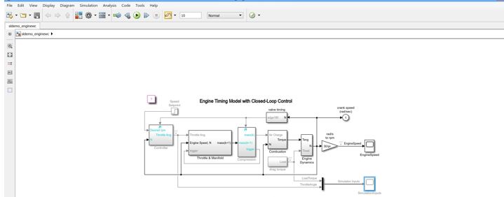
                                                      Fig-20 Engine Timing Model With
                                                 Closed Loop control

Conssisting of :1-Contrôler- Controler (ECU, ECU2, ECM, UBM,….,…)

                       2- Speed Setting and settling Point

                       3- Throttle And Manifold

                       4- Compression

                       5- Combustion

                       6- Valve Timing and Delay

                       7- Engine Dynamics

                       8- Crank Speed

                       9-Scope to show Speed and Closed Loop outputs

                                                           Fig-21 Engine Speed

                                          Fig-22 Engine Speed and Timing Control

Fig-23 Controller Designing Control system

Fig-24 Air Intake System

Fig-25 Engine Dynamics

Thank you hope you can use these applications in this fields and developping more and more For electrical and electronic, automatic control engineers.

See you in the next levels Having Fruits 30% 70% and 100% My Freinds.